Bangalore

Have you ever wondered where the centre of a city is? Where do those milestones you see on a highway which tend to (->) 0 actually reach 0? How does GPS measure distances? Well, I took it upon myself to find out!

What other city than our Bangalore? namma Bengaluru?

I wanted to figure out where the centre of Bangalore / Bengaluru is! I searched for Google for the Lat/ Long Co-ordinates of this great city – this is what I found

bangalore_01

Brilliant, so she is at a Latitude of 12.9716 and a Longitude of 77.5946.

Now, let us Plot!

I am using the map visualization package called ‘leaflet’ to plot. More details on this package at this link.

It is not a lot of code to plot using the leaflet package, a snapshot of RStudio with the code and the generated plot below –

bangalore_02

Look at the location, are you surprised? Well, I was. I was expecting it to be at the junction of old city (Chickpet) or some place near City Market or Chamarajpet!

If someone from the future were to communicate to you (from another dimension using say Gravity 🙂 Interstellar style) and ask you to be in the centre of Bangalore, now you know where to wait! You just need to know when!

bangalore_03


Word Cloud in R – Mythological Twist – Part II


Following the wonderful feedback I got on my previous post (WordCloud in R – Mythological twist), I thought I could do a similar text analysis on the other great Indian Epic, the Mahabharata!

This time it is bigger, a 5818 page, 14 MB pdf. The translation in question is the original translation from Kisari Mohan Ganguli which was done sometime between 1883 and 1896.

About the Mahabharata

The Mahabharata is an epic narrative of the Kurukshetra War and the fates of the Kaurava and the Pandava princes.

The Mahabharata is the longest known epic poem and has been described as “the longest poem ever written”. Its longest version consists of over 100,000 shlokas or over 200,000 individual verse lines (each shloka is a couplet), and long prose passages. About 1.8 million words in total, the Mahabharata is roughly ten times the length of the Iliad and the Odyssey combined, or about four times the length of the Ramayana.

The first section of the Mahabharata states that it was Ganesha who wrote down the text to Vyasa’s dictation. Ganesha is said to have agreed to write it only if Vyasa never paused in his recitation. Vyasa agrees on condition that Ganesha takes the time to understand what was said before writing it down.

The Epic is divided into a total of 18 Parvas or Books.

Well, if Rama was at the centre of Ramayana, who was the equivalent in Mahabharata? Krishna? One of the Pandavas? One of the Kauravas? Dhritarashtra? Or one of the queens – Draupadi? Kunti? Gandhari?

Let us find out –

Since, this is a continuation to the first blog in this series, I would not take you through the intricacies of downloading and installing packages. Also, there is a Rpdf that needs to be installed, you could lookup on the instructions in this link.

Download and copy the pdf onto a folder in the local file system. You may want to read the pdf in its entirety to a corpus.

mahabharata <- Corpus(URISource(files), readerControl = list(reader = Rpdf))

If I look at the environment variables, I can see the Corpus populated, which says it has 1 element and is of a 26.8 MB size.

wordcloud01

You could have a look at the details using ‘Inspect’

wordcloud02

Now, we can begin processing this text, firstly create a content transformer to remove any take a value and replace it with white-space.

> toSpace <- content_transformer(function(x, pattern) {return (gsub(pattern, " ", x))})

use this to eliminate colons and hyphens

> mahabharata <- tm_map(mahabharata, toSpace, "-")
> mahabharata <- tm_map(mahabharata, toSpace, ":")

Next, we might need to apply some transformations on the text, to know the available transformations type getTransformations() in the R Console.

wordcloud03

we would then need to convert all the text to lower case

> mahabharata <- tm_map(mahabharata, content_transformer(tolower))

let us also remove punctuation and numbers

> mahabharata <- tm_map(mahabharata, removePunctuation)

> mahabharata <- tm_map(mahabharata, removeNumbers)

and the stopwords

> mahabharata <- tm_map(mahabharata, removeWords, stopwords("english"))

The next step would be to create a TermDocumentMatrix, a matrix that lists all the occurrences of words in the corpus. The DTM represents the documents as rows and the words as columns, if a word occurs in a particular document, the matrix entry corresponding to that row and column is 1 or it is a 0. Multiple occurrences are then added to the same count.

> dtm <- TermDocumentMatrix(mahabharata)
> m <- as.matrix(dtm)
> v <- sort(rowSums(m),decreasing=TRUE)
> d <- data.frame(word = names(v),freq=v)

wordcloud04

Looking at the frequencies of the words, we may need to remove certain words to distill the insights from the DTM, for e.g., words like “thou”, “thy”, “thee”, “can”, “one”, “the”, “and”, “like”…

> mahabharata <- tm_map(mahabharata, removeWords, c("the", "will", "like", "can"))

upon further refinement, let us look at the top 15 frequently appearing words

wordcloud05


Brilliant, Isn’t it after all about a great battle between sons to be a King?!


The next occurrences throw up some interesting observations.

  1. Yudhishthira
  2. Arjuna
  3. Drona
  4. Bhishma
  5. Karna

and Krishna, who is considered central to the Epic is at 8th of most mentioned characters in Mahabharata.

Let us generate the WordCloud from this

rplot02_mb


Source for content on the Mahabharata

WordCloud in R – Mythological twist

A WordCloud in R


Let Noble thoughts come to us from every side

 – Rigveda, I-89-i


Have you ever wondered what it would be to do a textual analysis of some ancient texts? Would it not be nice to ‘mine’ insights into Valmiki’s Ramayana? Or Veda Vyasa’s Mahabharata? The Ramayana arguably happened about 9300 years ago. In the Thretha yuga. The wiki for Ramayana.

The original Ramayana consists of seven sections called kandas, these have varying numbers of chapters as follows: Bala-kanda—77 chapters, Ayodhya-kanda—119 chapters, Aranya-kanda—75 chapters, Kishkindha-kanda—67 chapters, Sundara-kanda—68 chapters, Yuddha-kanda—128 chapters, and Uttara-kanda—111 chapters.

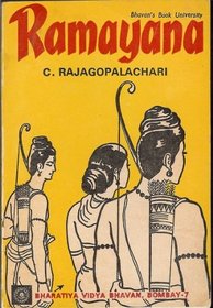
So, there are a total of 24,000 verses in total. Well, I don’t really have the pdf of the ‘Original’ version, I thought I could use C. Rajagopalachari’s English retelling of the epic. This particular book is quiet popular and has sold over a million copies. It is a page-turner and has around 300 pages.

Cover_Page

How about analyzing the text in this book?

Wouldn’t it be EPIC?!

That is exactly what I want to embark on this blog, text mining helps to derive valuable insights into the mind of the writer. It can also be leveraged to gain in-tangible insights like sentiment, relevance, mood, relations, emotion, summarization etc.

The first part of this series would be to run a descriptive analysis on the text and generate a word cloud. Tag clouds or word clouds add simplicity and clarity, the most used words are displayed as weighted averages, the more the count of the word, bigger would be the size of the word. After all, isn’t it visually engaging than looking at a table?

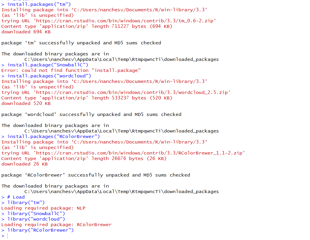
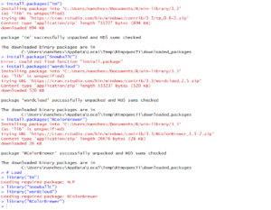
Firstly, we would need to install the relevant packages in R and load them –

WordCloud01

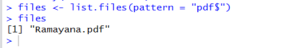
The second step would be to read the pdf (which is currently in my working directory)

I first validate if the pdf is there in my working directory

WordCloud02

The ‘tm’ package just provides a readPDF function, but the pdf engine needs to be downloaded. Let us use a pdf engine called xpdf. The link for setting up the pdf engine (and updating the system path) is here.

Great, now we can get rolling.

Let us create a pdf reader called ‘Rpdf’ using the code below, this instructs the pdftotext.exe to maintain the original physical layout of the text.

>  Rpdf <- readPDF(control = list(text = "-layout"))

Now, we might need to convert the pdf to text and store it in a corpus. Basically we need to instruct the function on which resource we need to read. The second parameter is the reader that we created in the previous line.

>  ramayana <- Corpus(URISource(files), readerControl = list(reader = Rpdf))

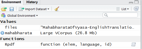
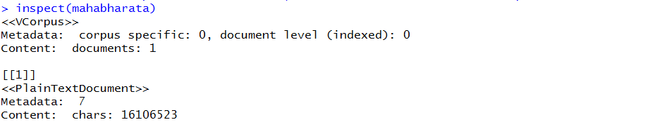
Now, let us check what the variable ‘ramayana’ contains

WordCloud03

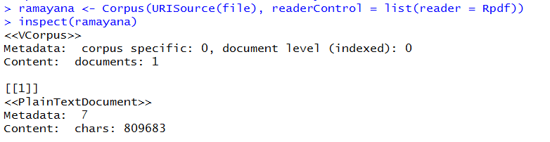
If I look at the summary of the variable, it will prompt me with the following details.

WordCloud04.bmp

The next step would be to do some transformation on the text, let us use the tm_map() function is to replace special characters from the text. We could use this to replace single quotes (‘), full stops (.) and replace them with spaces.

WordCloud05.bmp

Also, don’t you think we need to remove all the stop words? Words like ‘will’, ‘shall’, ‘the’, ‘we’ etc. do not make much sense in a word cloud. These are called stopwords, the tm_map provides for a function to do such an operation.

> ramayana <- tm_map(ramayana, removeWords, stopwords("english"))

Let us also convert all the text to lower

> ramayana <- tm_map(ramayana, content_transformer(tolower))

I could also specify some stop-words that I would want to remove using the code:

> ramayana <- tm_map(ramayana, removeWords, c("the", "will", "like", "can", "and", "shall")) 

Let us also remove white spaces and remove the punctuation.

> ramayana <- tm_map(ramayana, removePunctuation)
> ramayana <- tm_map(ramayana, stripWhitespace)

Any other pre-processing that you can think of? How about removing suffixes, removing tense in words? Is ‘kill’ different from ‘killed’? Do they not originate from the same stem ‘kill’? Or ‘big’, ‘bigger’, ‘biggest’? Can’t we just have ‘big’ with a weight of 3 instead of these three separate words? We use the stemDocument parameter for this.

> ramayana <- tm_map(ramayana, stemDocument)

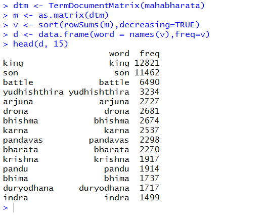
The next step would be to create a term-document matrix. It is a table containing the frequency of words. We use ‘termdocumentmatrix’ provided by the text mining package to do this.

> dtm <- TermDocumentMatrix(ramayana)
> m <- as.matrix(dtm)
> v <- sort(rowSums(m),decreasing=TRUE)
> d <- data.frame(word = names(v),freq=v)

Now, let us look at a sample of the words and their frequency we got. We pick the first 20.

WordCloud06.bmp

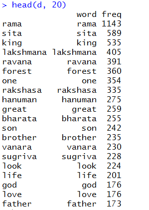
Not surprising, is it? ‘Rama’ is indeed the centre of the story.

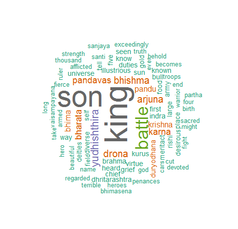
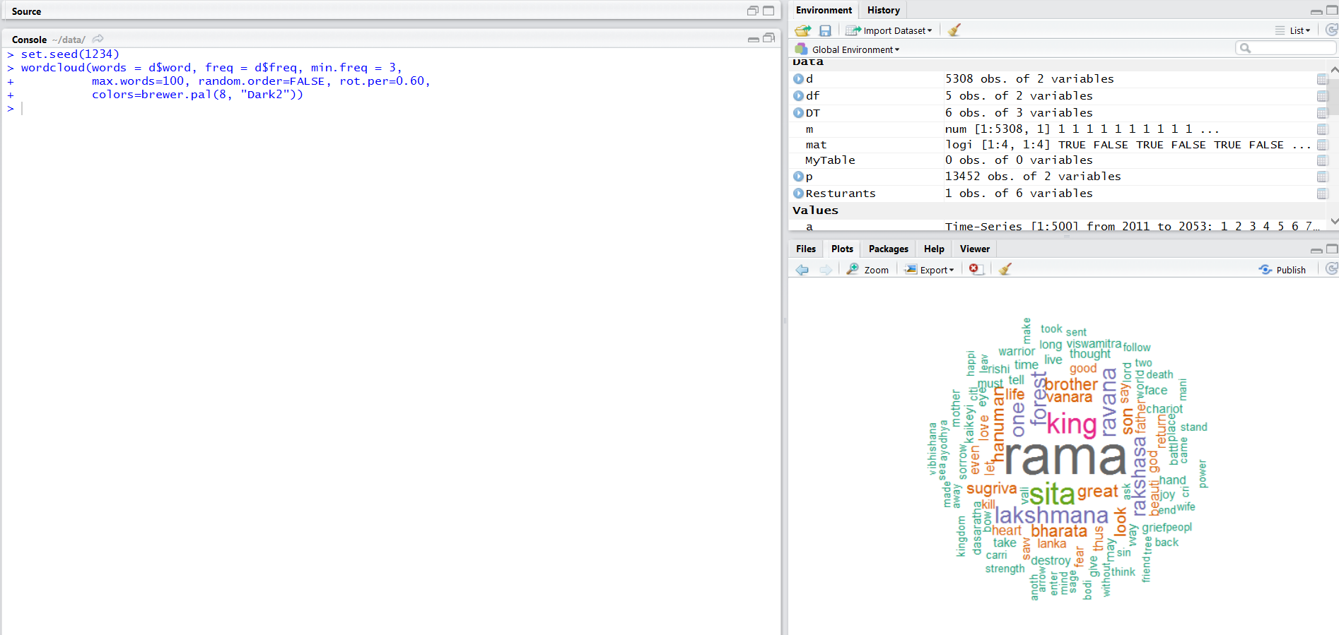
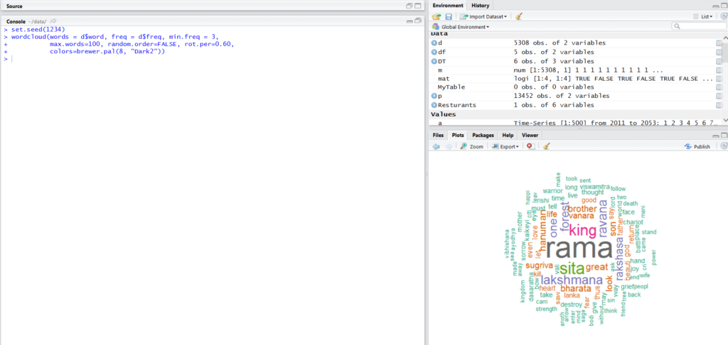
Now, let us generate the word cloud

> wordcloud(words = d$word, freq = d$freq, min.freq = 3, max.words=100, random.order=FALSE, rot.per=0.60,  colors=brewer.pal(8, "Dark2"))

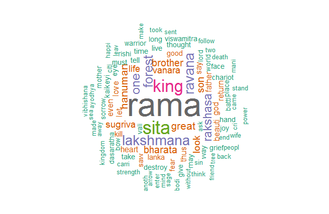
Voila!  The word cloud of all the words of Ramayana.

WordCloud07.bmp

A view of plot downloaded from R.

WordCloud08


If you like this, you could comment below. If you would like to connect with me, then be sure to find me on Twitter, Facebook, LinkedIn. The links are on the side navigation. Or you could drop an email to shivdeep.envy@gmail.com

Data Manipulation in R with dplyr

  • The R language is widely used among data scientists, statisticians, researchers and students.

    It is simply the leading tool for statistics, data analysis and machine learning. It is platform-independent, open-source, and has a large, vibrant community of users.

    The Comprehensive R Archive Network is the one-stop-shop for all R packages.

    This really brings us to the package to be discussed on this blog – dplyr. The CRAN documentation for dplyr can be found here.

    For this blog, I would be demonstrating the 5 operations of the package. The first thing we would need is to install the package and load the library.

    install.packages(“dplR”)

    > library(dplR)

    We then need to find a dataset on which we could run these operations. CRAN makes the download logs of their packages publicly available here – CRAN package download logs. Let us download the file for July 8, 2014 (we could really pick a log from any date) onto RStudio’s working directory.

    Once the file has been copied onto the working directory of R, execute the below line (where the variable path2csv stores the location of the csv)

    > mydf <- read.csv(path2csv, stringsAsFactors = FALSE)


    we then save the data frame onto a variable called cran by converting it to a tbl_df to improve readability. Calling the variable cran prints out the contents.

    > cran <- tbl_df(mydf)
    > cran


    Capture_Dplyr1.PNG

    The dplyr philosophy is to have small functions that do one thing well. There are basically 5 commands that cover most of the fundamental data manipulation tasks.

    • select()
    Usually in the entire data set that we use for analyis, we would really be interested in a few columns. This function is used to select / fetch the columns which are required. If I only need the columns ip_id, package and country. I execute the following statement –
    > select(cran, ip_id, package, country)

    CaptureDplyr2.PNG

    It is important to note that the columns are returned in the order in which we specified, irrespective of how it was in the original dataframe.
    We could also use the ‘-‘ sign to ommit the columns we do not need.
    > select(cran, -time)
    CaptureDplyr3.PNG
    
    • filter()
    Now that we know how to select columns, the next logical thing would be to be able to select rows. That is where the filter() function comes in.
    This is like the ‘where’ clause in SQL. Let us understand this by an example –
    > filter(cran, package == "swirl")

    CaptureDplyr4.PNG

    If you look at the column ‘package’, we now see that the resulting dataframe has only rows which have the package as ‘swirl’.
    Multiple conditions can be passed to filter() one after the other. For example, if I want to fetch all swirl packages downloaded on the OS – linux in India:
    > filter(cran, package == "swirl", r_os == "linux-gnu", country == "IN")

    CaptureDplyr5.PNG

    • arrange()
    This is used to order the rows of a dataset according to the values of a particular variable. Suppose we want to order all rows of a dataset in ascending / descending order of a column. Notice the ip_id column listed in descending order.
    > arrange(cran2, desc(ip_id))

    CaptureDplyr6.PNG

    • mutate()

    This function is used to edit or add additional columns to the dataframe. Suppose I want to convert the size column which is in bytes to megabytes and store the values in a column called size_mb.

    > mutate(cran3, size_mb = size / 2^20)

    CaptureDplyr7.PNG

    • sumarize()

    This function is used to collapse the dataset into a single row, the go-to function to calculate the mean in a sanitized dataframe.

    For example – I want to know the average download size from the size column.

    > summarize(cran, avg_bytes = mean(size))

    CaptureDplyr8.PNG

    sumarize() can also be used to fetch records in groups using the FOR EACH construct.
    Disclosure: The above example is from the dplyR lesson on the swirl package.