Text Mining – Shivdeep Nancherla

Following the wonderful feedback I got on my previous post (WordCloud in R – Mythological twist), I thought I could do a similar text analysis on the other great Indian Epic, the Mahabharata!

This time it is bigger, a 5818 page, 14 MB pdf. The translation in question is the original translation from Kisari Mohan Ganguli which was done sometime between 1883 and 1896.

About the Mahabharata

The Mahabharata is an epic narrative of the Kurukshetra War and the fates of the Kaurava and the Pandava princes.

The Mahabharata is the longest known epic poem and has been described as “the longest poem ever written”. Its longest version consists of over 100,000 shlokas or over 200,000 individual verse lines (each shloka is a couplet), and long prose passages. About 1.8 million words in total, the Mahabharata is roughly ten times the length of the Iliad and the Odyssey combined, or about four times the length of the Ramayana.

The first section of the Mahabharata states that it was Ganesha who wrote down the text to Vyasa’s dictation. Ganesha is said to have agreed to write it only if Vyasa never paused in his recitation. Vyasa agrees on condition that Ganesha takes the time to understand what was said before writing it down.

The Epic is divided into a total of 18 Parvas or Books.

Well, if Rama was at the centre of Ramayana, who was the equivalent in Mahabharata? Krishna? One of the Pandavas? One of the Kauravas? Dhritarashtra? Or one of the queens – Draupadi? Kunti? Gandhari?

Let us find out –

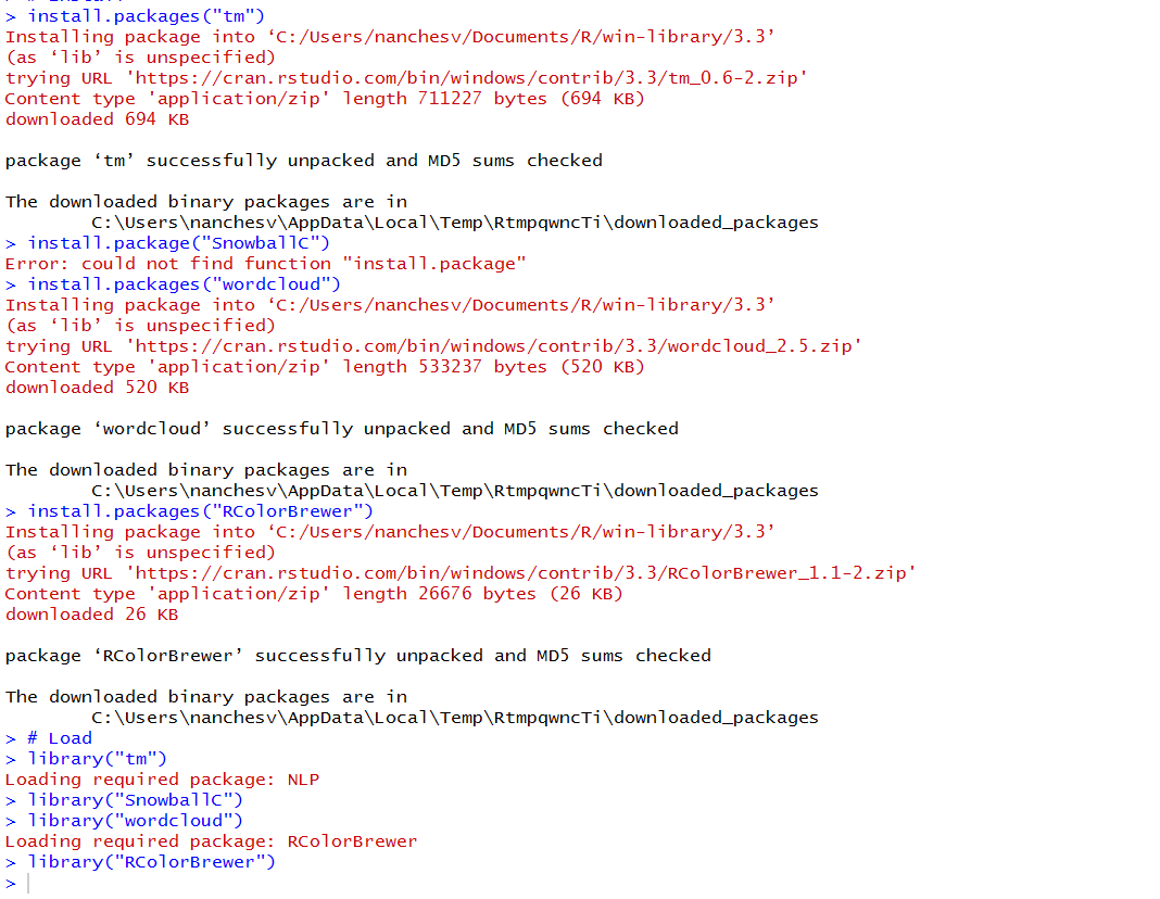
Since, this is a continuation to the first blog in this series, I would not take you through the intricacies of downloading and installing packages. Also, there is a Rpdf that needs to be installed, you could lookup on the instructions in this link.

Download and copy the pdf onto a folder in the local file system. You may want to read the pdf in its entirety to a corpus.

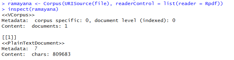
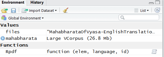
mahabharata <- Corpus(URISource(files), readerControl = list(reader = Rpdf))

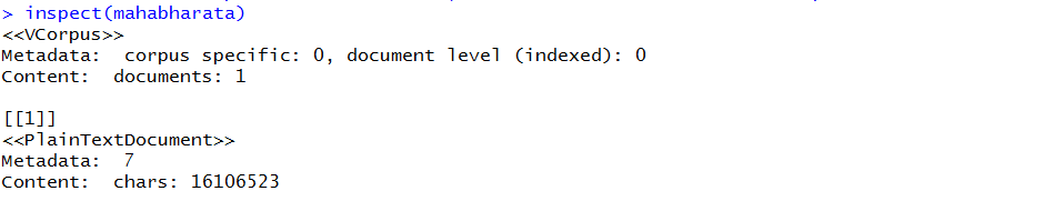
If I look at the environment variables, I can see the Corpus populated, which says it has 1 element and is of a 26.8 MB size.

You could have a look at the details using ‘Inspect’

Now, we can begin processing this text, firstly create a content transformer to remove any take a value and replace it with white-space.

> toSpace <- content_transformer(function(x, pattern) {return (gsub(pattern, " ", x))})

use this to eliminate colons and hyphens

> mahabharata <- tm_map(mahabharata, toSpace, "-")
> mahabharata <- tm_map(mahabharata, toSpace, ":")

Next, we might need to apply some transformations on the text, to know the available transformations type getTransformations() in the R Console.

we would then need to convert all the text to lower case

> mahabharata <- tm_map(mahabharata, content_transformer(tolower))

let us also remove punctuation and numbers

> mahabharata <- tm_map(mahabharata, removePunctuation)

> mahabharata <- tm_map(mahabharata, removeNumbers)

and the stopwords

> mahabharata <- tm_map(mahabharata, removeWords, stopwords("english"))

The next step would be to create a TermDocumentMatrix, a matrix that lists all the occurrences of words in the corpus. The DTM represents the documents as rows and the words as columns, if a word occurs in a particular document, the matrix entry corresponding to that row and column is 1 or it is a 0. Multiple occurrences are then added to the same count.

> dtm <- TermDocumentMatrix(mahabharata)
> m <- as.matrix(dtm)
> v <- sort(rowSums(m),decreasing=TRUE)
> d <- data.frame(word = names(v),freq=v)

Looking at the frequencies of the words, we may need to remove certain words to distill the insights from the DTM, for e.g., words like “thou”, “thy”, “thee”, “can”, “one”, “the”, “and”, “like”…

> mahabharata <- tm_map(mahabharata, removeWords, c("the", "will", "like", "can"))

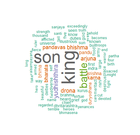
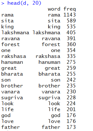
upon further refinement, let us look at the top 15 frequently appearing words

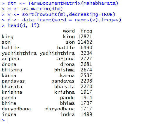
Brilliant, Isn’t it after all about a great battle between sons to be a King?!

The next occurrences throw up some interesting observations.

Yudhishthira
Arjuna
Drona
Bhishma
Karna

and Krishna, who is considered central to the Epic is at 8th of most mentioned characters in Mahabharata.

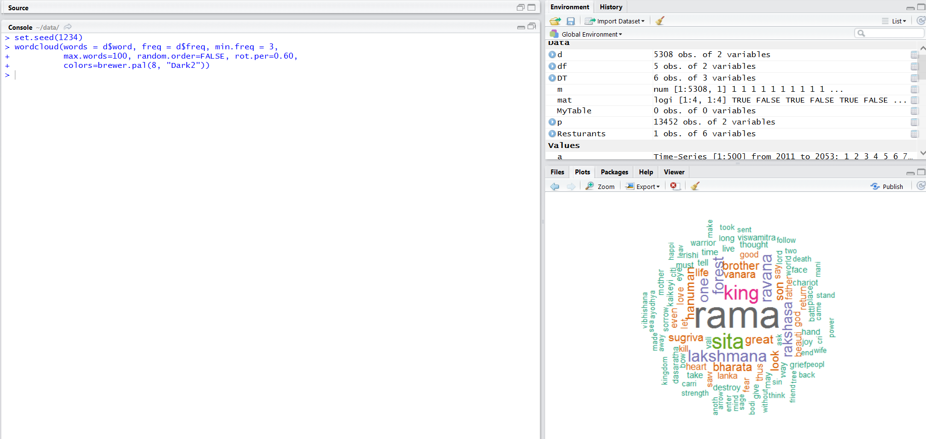
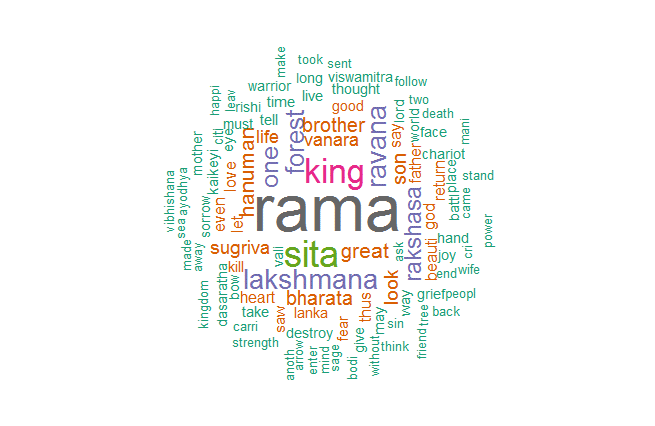
Let us generate the WordCloud from this

Source for content on the Mahabharata

A WordCloud in R

Let Noble thoughts come to us from every side

– Rigveda, I-89-i

Have you ever wondered what it would be to do a textual analysis of some ancient texts? Would it not be nice to ‘mine’ insights into Valmiki’s Ramayana? Or Veda Vyasa’s Mahabharata? The Ramayana arguably happened about 9300 years ago. In the Thretha yuga. The wiki for Ramayana.

The original Ramayana consists of seven sections called kandas, these have varying numbers of chapters as follows: Bala-kanda—77 chapters, Ayodhya-kanda—119 chapters, Aranya-kanda—75 chapters, Kishkindha-kanda—67 chapters, Sundara-kanda—68 chapters, Yuddha-kanda—128 chapters, and Uttara-kanda—111 chapters.

So, there are a total of 24,000 verses in total. Well, I don’t really have the pdf of the ‘Original’ version, I thought I could use C. Rajagopalachari’s English retelling of the epic. This particular book is quiet popular and has sold over a million copies. It is a page-turner and has around 300 pages.

How about analyzing the text in this book?

Wouldn’t it be EPIC?!

That is exactly what I want to embark on this blog, text mining helps to derive valuable insights into the mind of the writer. It can also be leveraged to gain in-tangible insights like sentiment, relevance, mood, relations, emotion, summarization etc.

The first part of this series would be to run a descriptive analysis on the text and generate a word cloud. Tag clouds or word clouds add simplicity and clarity, the most used words are displayed as weighted averages, the more the count of the word, bigger would be the size of the word. After all, isn’t it visually engaging than looking at a table?

Firstly, we would need to install the relevant packages in R and load them –

The second step would be to read the pdf (which is currently in my working directory)

I first validate if the pdf is there in my working directory

The ‘tm’ package just provides a readPDF function, but the pdf engine needs to be downloaded. Let us use a pdf engine called xpdf. The link for setting up the pdf engine (and updating the system path) is here.

Great, now we can get rolling.

Let us create a pdf reader called ‘Rpdf’ using the code below, this instructs the pdftotext.exe to maintain the original physical layout of the text.

>  Rpdf <- readPDF(control = list(text = "-layout"))

Now, we might need to convert the pdf to text and store it in a corpus. Basically we need to instruct the function on which resource we need to read. The second parameter is the reader that we created in the previous line.

>  ramayana <- Corpus(URISource(files), readerControl = list(reader = Rpdf))

Now, let us check what the variable ‘ramayana’ contains

If I look at the summary of the variable, it will prompt me with the following details.

The next step would be to do some transformation on the text, let us use the tm_map() function is to replace special characters from the text. We could use this to replace single quotes (‘), full stops (.) and replace them with spaces.

Also, don’t you think we need to remove all the stop words? Words like ‘will’, ‘shall’, ‘the’, ‘we’ etc. do not make much sense in a word cloud. These are called stopwords, the tm_map provides for a function to do such an operation.

> ramayana <- tm_map(ramayana, removeWords, stopwords("english"))

Let us also convert all the text to lower

> ramayana <- tm_map(ramayana, content_transformer(tolower))

I could also specify some stop-words that I would want to remove using the code:

> ramayana <- tm_map(ramayana, removeWords, c("the", "will", "like", "can", "and", "shall"))

Let us also remove white spaces and remove the punctuation.

> ramayana <- tm_map(ramayana, removePunctuation)
> ramayana <- tm_map(ramayana, stripWhitespace)

Any other pre-processing that you can think of? How about removing suffixes, removing tense in words? Is ‘kill’ different from ‘killed’? Do they not originate from the same stem ‘kill’? Or ‘big’, ‘bigger’, ‘biggest’? Can’t we just have ‘big’ with a weight of 3 instead of these three separate words? We use the stemDocument parameter for this.

> ramayana <- tm_map(ramayana, stemDocument)

The next step would be to create a term-document matrix. It is a table containing the frequency of words. We use ‘termdocumentmatrix’ provided by the text mining package to do this.

> dtm <- TermDocumentMatrix(ramayana)
> m <- as.matrix(dtm)
> v <- sort(rowSums(m),decreasing=TRUE)
> d <- data.frame(word = names(v),freq=v)

Now, let us look at a sample of the words and their frequency we got. We pick the first 20.

Not surprising, is it? ‘Rama’ is indeed the centre of the story.

Now, let us generate the word cloud

> wordcloud(words = d$word, freq = d$freq, min.freq = 3, max.words=100, random.order=FALSE, rot.per=0.60,  colors=brewer.pal(8, "Dark2"))

Voila! The word cloud of all the words of Ramayana.

A view of plot downloaded from R.

If you like this, you could comment below. If you would like to connect with me, then be sure to find me on Twitter, Facebook, LinkedIn. The links are on the side navigation. Or you could drop an email to shivdeep.envy@gmail.com

Category: Text Mining

Word Cloud in R – Mythological Twist – Part II

About the Mahabharata

WordCloud in R – Mythological twist

A WordCloud in R